| Crash course to Maple |
| Crash course to Maple |
This page presents to you the most important Maple commands and functions available, so that you can try out Maple's capabilities even if you have not yet worked with this system before.
Indeed, it is an introduction on the fast run; if you like to use Maple regularly and in all its aspects, it is inevitable studying the online help and books.
You can use this course with Maple 6 and 7, and also in Maple V Release 3, 4, and 5 (see remarks).
You can switch between neighboring input lines by using the keys Up and Down.
The cursor keys left and right allow you to move in an input line.
You can insert characters with the INS or delete them with DEL keys.
Expressions or parts of them can be copied to the clipboard using CTRL+C and be pasted with CTRL+V at any position.
Inputs are terminated with a semicolon (except when calling the online help), by pressing the RETURN key Maple computes the result and displays it.
![[Maple Bitmap]](mpl7crashcourse/mapleonthefastone1.gif)
Mark a file that you want to open:
![[Maple Bitmap]](mpl7crashcourse/mapleonthefastone2.gif)
To save a worksheet so that you can use it in another session, click on the `File` menu and then choose the `Save As` item.
![[Maple Bitmap]](mpl7crashcourse/mapleonthefastone3.gif)
Specify a file name and then press the `Save` button.
![[Maple Bitmap]](mpl7crashcourse/mapleonthefastone4.gif)
| Basic operators | |
| addition | + |
| subtraction | - |
| multiplication | * |
| division | / |
| exponentiation | ^ |
| Elementary functions | |
| Square root | sqrt(x) or x^(1/2) |
| nth root | surd(x, n) or x^(1/n) |
| Exponential function to the base e=2.7182818... | exp(x) |
| Logarithm to the base a | log[a](x) |
| Natural logarithm | ln(x) |
| Trigonometric functions | sin(x), cos(x), tan(x), sec(x), cot(x), csc(x) |
| Hyperbolic functions | sinh(x), cosh(x), tanh(x), sech(x), csch(x), coth(x) |
| Inverse trigonometric functions | arcsin(x), arccos(x), arctan(x), arcsec(x), arccsc(x), arccot(x) |
| Inverse hyperbolic functions | arcsinh(x), arccosh(x), arctanh(x), arcsech(x), arccsch(x), arccoth(x) |
| Absolute value | abs(x) |
| Sign | sgn(x) |
Maple knows general precedences, e.g. 3*4 + 1 = 12 + 1 = 13, but 3 * (4+1) = 3 * 5 = 15. In Maple, as in mathematics, almost all other programming languages and with pocket calculators, use brackets to set other precedences.
Your first Maple example:
> 3*4+1;
13
> 3*(4+1);
15
> x^2-2*x+1;
![]()
You can store this expression in a variable, so that you can refer to it in session again and again by calling its name. Allocate expressions to a variable - here p - by using the characters :=, a colon directly followed by an equals sign.
> p := x^2-2*x+1;
![]()
Displaying the graph is often very helpful to estimate characteristics and behavior. The most basic plotting function is plot.
> plot(p, x);
![[Maple Plot]](mpl7crashcourse/mapleonthefastone7.gif)
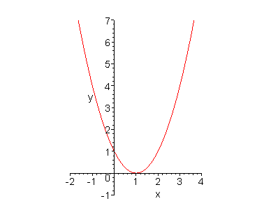
This means that the expression p in the unknown x is plotted. By default, Maple uses the x-range -10 .. 10. Specify another interval over the x-axis, e.g. the interval [-2, 4]:
> plot(p, x=-2 .. 4);
![[Maple Plot]](mpl7crashcourse/mapleonthefastone8.gif)
Note that in Maple, the boundaries are separated by two dots (..). You can also specify the y-range:
> plot(p, x=-2 .. 4, y=-1 .. 7);
![[Maple Plot]](mpl7crashcourse/mapleonthefastone9.gif)
The plot function accepts a lot of so-called plot options, one of the most important is scaling=constrained, which tells Maple to use equal x- and y-ranges.
> plot(p, x=-2 .. 4, y=-1 .. 7, scaling=constrained);

For other plot options, check:
> ?plot,options
> factor(p);
![]()
Multiply out the result with expand, thus regaining the original polynomial. To specify the last result Maple has computed, use the percentage sign. (In Maple V Release 4 and earlier versions, use the quotation mark " instead of %.)
> expand(%);
![]()
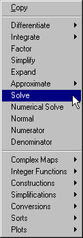
solve determines solutions to equations. To get the roots of p, specify the equation as the first, and the indeterminate in p as the second argument.
> solve(p=0, x);
![]()
Maple returns the solution twice for if you convert p to linear factors, you get two zeros -1: x2-2*x+1 = (x-1)*(x-1).
If you want to receive numerical values, use subs. To determine the value of p at point x=0, enter:
> subs(x=0, p);
![]()
You can also directly assign values to variables such as x:
> x := 0;
![]()
Thus Maple automatically returns:
> p;
![]()
However, p is no longer available as the symbolic expression x2-2x+1, but as the numerical value 1. If you want to do further computation with the original symbolic polynomial p = x2-2x+1, you have to reset/unassign x:
> x := 'x';
![]()
> p;
![]()
Suppose you have two equations:
> eq1 := 3*x-2*y=8;
eq1 := 3 x - 2 y = 8
> eq2 := 5*x-3*y=4;
eq2 := 5 x - 3 y = 4
Pass the two equations in one set as the first argument, and the variables to be solved for as another set to solve:
> solve({eq1, eq2}, {x, y});
{y = -28, x = -16}
> simplify(sin(x)^2+2*cos(x)^2);
![]()
You can isolate variables in an equation (in Maple V Release 5 and before you first have to initialize this command by typing readlib(isolate): at the command prompt).
> isolate(x*y+2=0, y);
![]()
collect collects all the coefficients with the same rational power of an indeterminate together:
> collect(5*x + a*x + 1, x);
(5 + a) x + 1
normal seeks for the common denominator:
> normal((2*x-1)/(x-2)-(x+1)/(x+2));
![]()
Hint: To easily execute manipulations, right-click into the output (the fraction) and choose the desired action (this works with Maple V Release 5.X and later versions):

> f := x -> (x+1)*(x-1);
f := x -> (x + 1) (x - 1)
You can apply all Maple functions to self-defined functions:
> expand(f(x));
![]()
To get function values, pass arguments (here: x-values):
> f(1);
0
> f(2);
3
Note that Maple is a symbolic computer algebra system. You can either enter floating point values like in a pocket calculator and receive floating point results,
> f(0.5);
-.75
or use symbolic values such as a fraction and get an accurate, symbolic result.
> f(1/2);
![]()
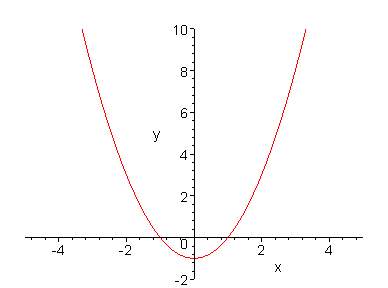
Defining a function prevents you from using the eval function. Plots:
> plot(f(x), x=-5 .. 5, y=-2 .. 10);

Interceptions with the line y=2:
> solve(f(x)=2, x);
![]()
You can also print a table of function values using a for-loop. Here, all function values in the interval [-2, 2] (from -2 to 2) with step (step) 0.5 are printed:
> for i from -2 to 2 by 0.5 do
> f(i)
> od;
3
1.25
-0.
-.75
-1.
-.75
0.
1.25
3.00
You can also print the x-values (here expressed by the loop variable i) along with the function values:
> for i from -2 to 2 by 0.5 do
> i, f(i)
> od;
-2, 3
-1.5, 1.25
-1.0, -0.
-.5, -.75
0., -1.
.5, -.75
1.0, 0.
1.5, 1.25
2.0, 3.00
> limit((x^2-1)/(x-1), x=1);
![]()
The behavior in the infinite is determined by passing the constant infinity instead of a point.
> limit(n/(n+1), n=infinity);
![]()
diff computes the (first) derivative.
> g := x^3-x^2-x-1;
![]()
> diff(g, x);
![]()
As with all other Maple commands, you can apply diff to the output again (in Maple V Release 4 and earlier, use the double quote " instead of the percentage sign).
> diff(%, x);
![]()
For the nth derivative, put a dollar sign and the integer n behind the indeterminate, for the 2nd derivative:
> diff(g, x$2);
![]()
For the 3rd derivative:
> diff(g, x$3);
![]()
Integration/anti-differentiation is performed with int:
> int(g, x);
![]()
int also determines the area under a curve between two points. Pay attention to the two dots separating the boundaries.
> int(g, x=1 .. 3);
![]()
Series expansion of an expression at a point:
> series(sin(x), x=0);
![]()
Differential equations are solved with the dsolve function. The diff function is used to define the differential equation:
> ode := diff(y(x), x) = 2*x;
![]()
> dsolve(ode, y(x));
![]()
Initial values can be given by passing both the ODE and the value as a set in curly brackets.
> dsolve({ode, y(0)=1}, y(x));
![]()
> restart:
The linalg package contains a lot of functions that allow you to work with vectors and matrices. You have to initialize this package before using its functions:
> with(linalg):
Vectors are defined with the vector functions.
> v1 := vector([1, 2, 3]);
v1 := [1, 2, 3]
> v2 := vector([a, b, c]);
v2 := [a, b, c]
You can add and suctract these vectors with the evalm command:
> evalm(v1 + v2);
[1 + a, 2 + b, 3 + c]
> evalm(v1 - v2);
[1 - a, 2 - b, 3 - c]
Dot product:
> dotprod(v1, v2);
a + 2 b + 3 c
Cross product:
> crossprod(v1, v2);
[2 c - 3 b, 3 a - c, b - 2 a]
Multiplication of a vector and a scalar:
> scalarmul(v1, s);
[s, 2 s, 3 s]
Matrices are defined with the matrix command.
> A := matrix([[a, b], [c, d]]);
![A := _rtable[3026604]](mpl7crashcourse/mapleonthefastone39.gif)
> B := matrix([[e, f], [g, h]]);
![B := _rtable[3105484]](mpl7crashcourse/mapleonthefastone40.gif)
Addition:
> evalm(A + B);
![_rtable[3189060]](mpl7crashcourse/mapleonthefastone41.gif)
Subtraction:
> evalm(A - B);
![_rtable[3056596]](mpl7crashcourse/mapleonthefastone42.gif)
Non-communitative multiplication is performed with the &* operator, whereas scalar multiplication is done with the multiplication operator *.
> evalm(A &* B);
![_rtable[2616420]](mpl7crashcourse/mapleonthefastone43.gif)
> evalm(A * s);
![s*_rtable[3026604]](mpl7crashcourse/mapleonthefastone44.gif)
Determinant:
> det(A);
![]()
Lets define a new matrix A, you do not have to restart Maple or unassign A before:
> A := matrix([
> [1, -3, 1.5, -1],
> [-2, 1, 3.5, 2],
> [1, -2, 1.2, 2],
> [3, 1, -1, -3]
> ]);
![A := _rtable[2926164]](mpl7crashcourse/mapleonthefastone46.gif)
> c := vector([-10.4, -16.5, 0, -0.7]);
c := [ -10.4, -16.5, 0, -.7 ]
To get solutions to a system of equations, apply the linsolve function:
> linsolve(A, c);
[ .8079999992, -.184000001, -5.879999999, 2.939999998 ]
Type
> ?newuser,usermenu
in the input line for the `Maple New User's Tour Main Menu`. As opposed to statements, when calling the online help, do not terminate the input with a semicolon.
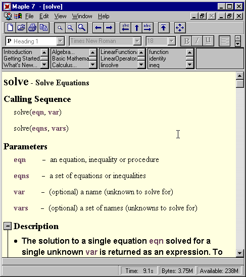
If you would like to have more information on a specific Maple function, e.g. the solve command to determine solutions, type:
> ?solve

In general:
> ?command
Also try have a look at the `Help menu item`, it features the entries `Topic Search` and `Full Text Search`. After entering the term or keyword, press the `OK` button.


![]()